# Use blending to reaggregate data
Reaggregation is a common need in data visualization. This article will help you understand the concept of reaggregation and how to achieve it in Insights using data blending.
One example of reaggregation is calculating the **average of averages**. For example, say you have a table of stock price changes:
| **Sector** | **Ticker** | **Price Change** |
| ---------- | ---------- | ---------------- |
| Tech | GOOG | +6 |
| Tech | AAPL | +5 |
| Tech | MSFT | -3 |
| Tech | NFLX | -1 |
| Energy | E1 | +2 |
| Energy | E2 | +10 |
| Energy | E3 | -3 |
| Finance | F1 | -6 |
The average price change for this data is a simple aggregation.
| **Average of Price Change** |
| --------------------------- |
| **1.25** |
To calculate the average price change for every sector, you'd group this table by the *Sector* dimension.
| **Sector** | **Average of Price Change** |
| ---------- | --------------------------- |
| Tech | **1.75** |
| Energy | **3** |
| Finance | **-6** |
To reaggregate this data, you'd apply another aggregation function, for example, applying average again:
| **Average of Average of Price Change** |
| -------------------------------------- |
| **-0.42** |
### **Reaggregation in Insights**
To reaggregate metrics in Insights, use [data blending](https://docs.antsomi.com/cdp-365-user-guide-en/insights/reports/blend-multiple-data-sources-in-a-chart/broken-reference). Blending lets you work around the fact that previously aggregated fields are set to the AUTO field type. You can't change this field type, nor can you apply another aggregation function to such fields.
For example, to find the average change of stock prices per sector in Insights, you'd create a blend configuration that joins the same data source with itself. Use *Sector* as the join key, and include the *Average Price Change* metric in both the left and right data sources, as shown below:
Data blending example
*Sector**Average Price Change*This blended data source lets you apply new aggregations on the previously aggregated *Price Change* field.
**Blending disaggregates data**
Blending data creates a new table from the columns that you select in the blend configuration. Metrics in the new table are treated as unaggregated numbers.Because *Price Change* is no longer an aggregated metric, you can now apply a new aggregation function on it. The table below shows the results of creating a new metric AVG(*Price Change*) with the previously aggregated numbers:
Average price change
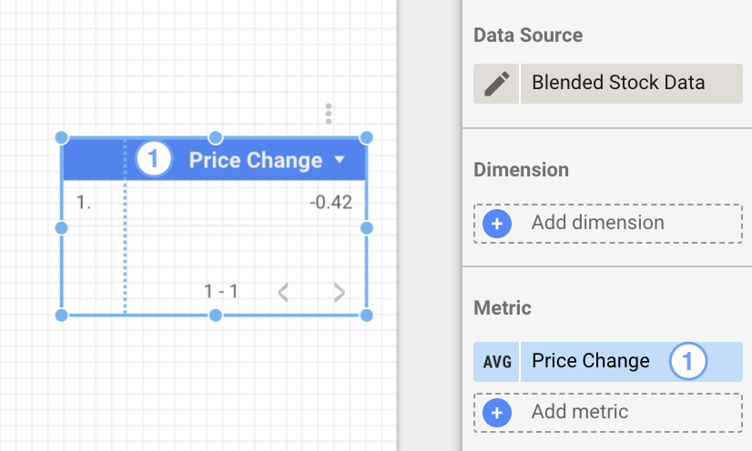
 *Price Change*
This new metric reaggregates the numbers **1.75, 3** and **-6** and displays their average: **-0.42** .
### Create a ratio column using blending
Another use for blending is to create ratio metrics with already aggregated numbers. Say you want to create a ratio column that divides one metric by another.
In this example, we'll use two fields; *Clicks* and *Impressions*, coming from two different data sources.
| **Website** | **Clicks** |
| ------------ | ---------- |
| google.com | 300 |
| facebook.com | 400 |
| twitter.com | 200 |
| **Website** | **Impressions** |
| ------------ | --------------- |
| google.com | 2000 |
| facebook.com | 2500 |
| twitter.com | 2000 |
You can create a ratio column with a calculated field *Clicks/Impressions* by blending these two data sources.
| **Website** | **Clicks** | **Impressions** | **Clicks / Impressions** |
| --------------- | ---------- | --------------- | ------------------------ |
| google.com | 300 | 2000 | 0.15 |
| facebook.com | 400 | 2500 | 0.16 |
| twitter.com | 200 | 2000 | 0.1 |
| **Grand Total** | 900 | 6500 | **0.41** |
All the rows of *Clicks/Impressions* have correct information except the summary row which shows the sum of the ratio column **`SUM(`*****`Clicks / Impressions`*****`)`**. This happens because *Clicks/Impressions* is calculated for each row \[0.15, 0.16, 0.1] and then the `SUM` function is applied to it. \[0.15 + 0.16 + 0.1 = 0.41].
The correct result is **900/6500 = 0.14 .**You can do this by calculating the ratio column values using the formula **`SUM(`*****`Clicks`*****`) / SUM(`*****`Impressions`*****`)`.**
| **Website** | **Clicks** | **Impressions** | **SUM(Clicks) / SUM(Impressions)** |
| --------------- | ---------- | --------------- | ---------------------------------- |
| google.com | 300 | 2000 | 0.15 |
| facebook.com | 400 | 2500 | 0.16 |
| twitter.com | 200 | 2000 | 0.1 |
| **Grand Total** | 900 | 6500 | **0.14** |
In this case, the summary row shows **`SUM( SUM(`*****`Clicks`*****`) / SUM(`*****`Impressions`*****`) )`. `SUM(`*****`Clicks`*****`)`** \[900] is divided by **`SUM(`*****`Impressions`*****`)`**\[6500] to give **0.14.** The **`SUM`** function is then applied to it again. The result is still **0.14**.

